Fast(er) ai
Jeremy Howard’s fast.ai Study Group, Q1 2018
In February, I was invited by Sydney Machine Learning’s Paul Conyngham, to join a Saturday morning study group to tackle the first seven weeks of Jeremy Howard’s fast.ai Deep Learning for Coders MOOC, under the kind auspices of The Domain Group. I was excited to be part of the study group, as the course came highly recommended by my mentor Greg Baker.
In this ongoing post I will try to document everything I learned. While we studied the material together, the Jupyter notebooks here represent my own work at extending concepts covered in the MOOC with kaggle sourced datasets and competitions. The course uses the fast.ai library as a wrapper for PyTorch an open source, GPU optimized library for deep learning, developed by Facebook’s AI team.
Week 1: Facial Recognition Classifier - Tony Stark or Elon Musk?
Robert Downey Jr reinvigorated his career with his portrayal of Tony Stark in Marvel’s Iron Man (2008) movies. A little known fact is that Downey (hereafter: RDJ) based his portrayal of the genius, billionaire, playboy, philanthropist on serial entrepreneur Elon Musk. I wanted to use a Convolutional Neural Network, trained on ImageNet data to train a single label image classification model to distinguish between photos of RDJ and Elon Musk.
The input for this convolutional neural network will be photos of Elon Musk and Robert Downey Jr. Each photo will be transformed into a rank 3 tensor with dimensions height x width x 3 where 3 represents each of the Red, Blue and Green channels that combine to form a pixel color. Each pixel in an image will have a value from 0 (black) to 255 (white).
Our output activation layer for this Convolutional Neural Network will be a sigmoid function which transforms the result of the previous layer into a 0 (RDJ) or 1 (Musk) classification, based on a preset threshold. Here we use the threshold 0.5, meaning that any image which is processed by the penultimate layer of our CNN and has an output value greater than or equal to 0.5 will be assigned to Musk otherwise Downey.
Figure 1: Rank Tensor 3 representation of Elon Musk’s photo
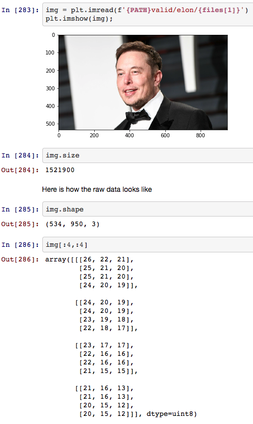
I use the Resnet34 architecture for facial recognition based on the paper by He et al (2015), trained for 10 epochs with a learning rate = 0.01, pre-trained on the ImageNet database. The learning rate is a hyperparameter representing how quickly or how slowly we want to update the weights of our model.
A first pass using this model reveals the images that the architecture is more sure about
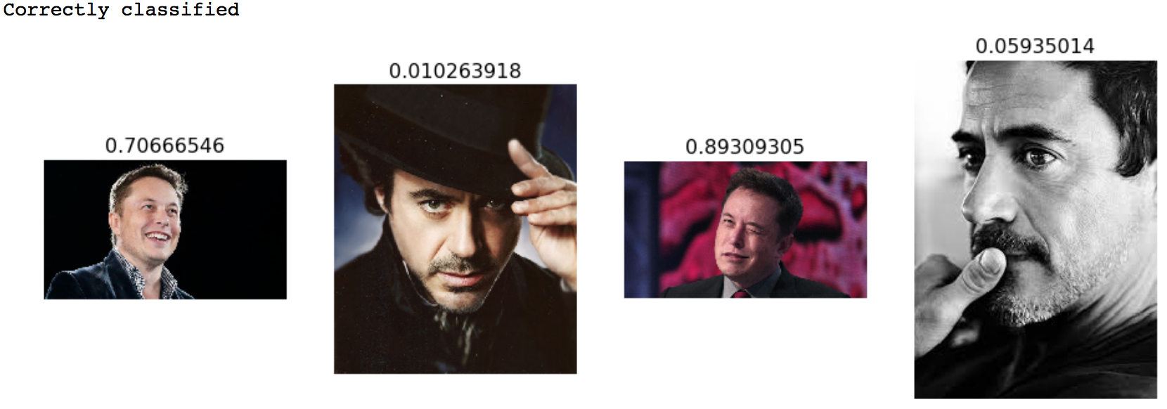
and the images it’s not quite so sure about. Note that the architecture seems to be having a tougher time identifying Elon as opposed to Downey. The model has an accuracy of around 70%.

We’re going to make a few quick improvements to the Resnet30 model by:
- Changing the learning rate - this is our key hyperparameter
- Augmenting the data
In order to determine the ideal learning rate, we use the he technique developed in the 2015 paper Cyclical Learning Rates for Training Neural Networks, where we keep increasing the learning rate from a very small value, until the loss stops decreasing. We can plot the learning rate across batches to see what this looks like.
Figure 2: Chart of Learning Rate
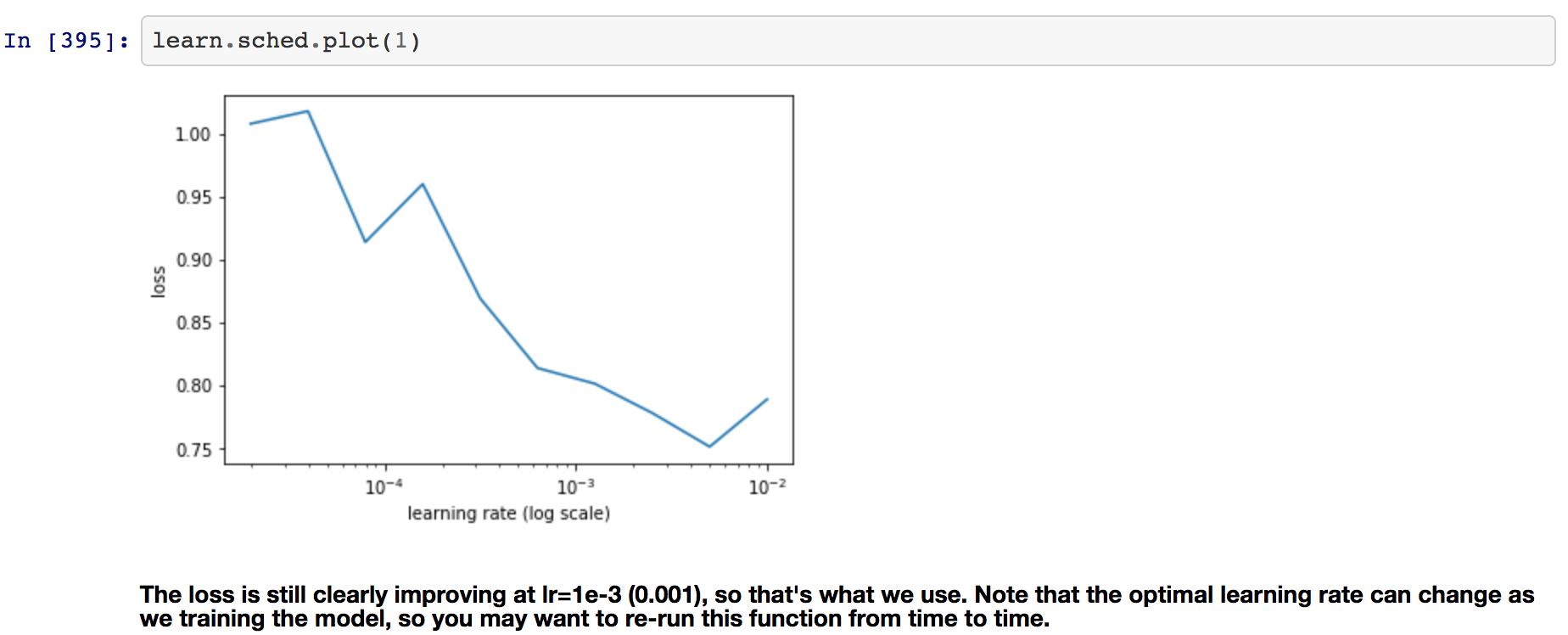
For our untrained model, we start with a learning rate = 0.001 at which point the loss is clearly improving and not yet at a minimum. Simply changing the learning rate and training for more epochs will result in overfitting. One way to fix this is to effectively create more data, through data augmentation. This refers to randomly changing the images in ways that shouldn’t impact their interpretation, such as horizontal flipping, zooming, and rotating.
Figure 3: Augmenting the Images
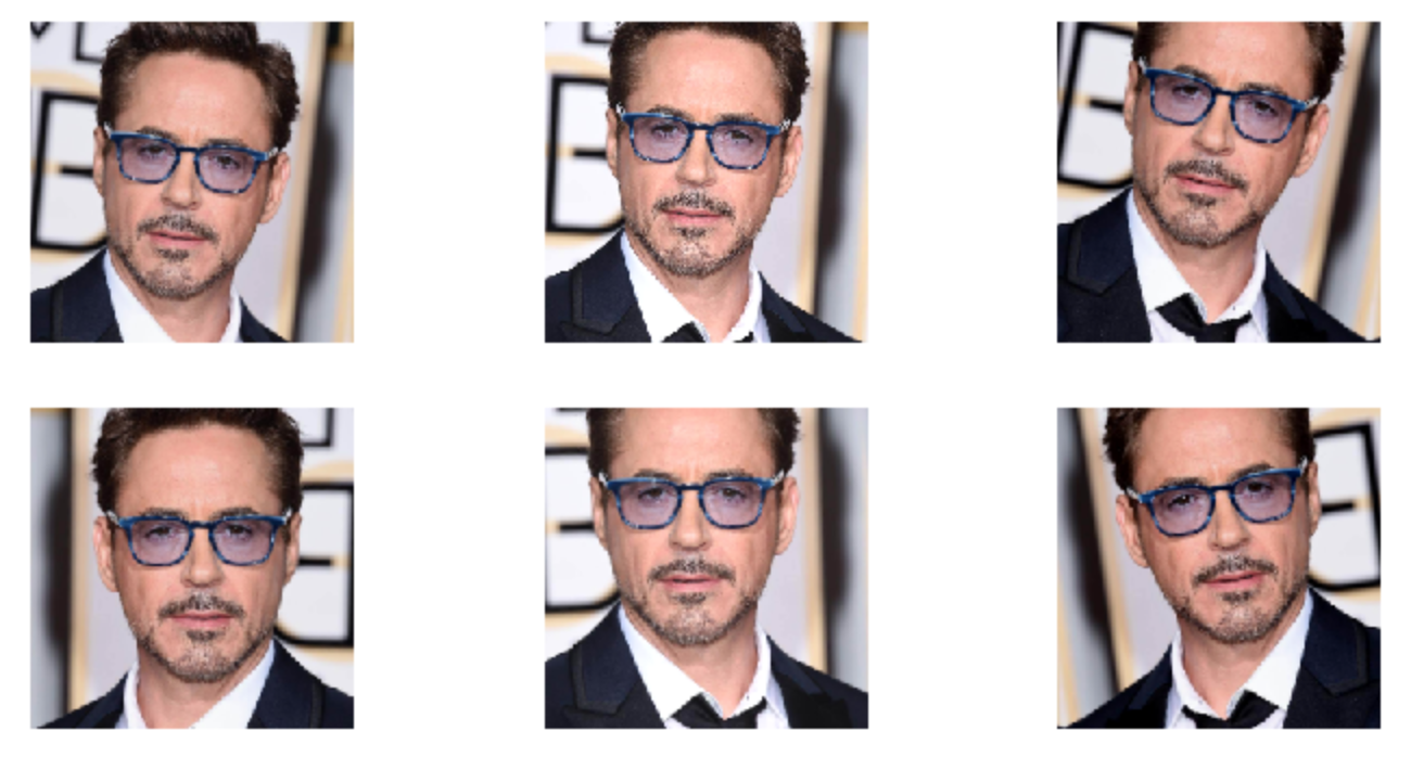
This is similar to bootstrapping where we create new pieces of data using the same distribution of the original data. Now we re-train the model using our new learning rate and by adding our augmented data with the training model. We augment an image by taking the original image and slightly transforming it by tilting it to the left and right. As convolutional neural networks architectures such as ResNet34 have been trained on Facial Images, we apply side-on transforms as shown in Figure 3 to generate more data.
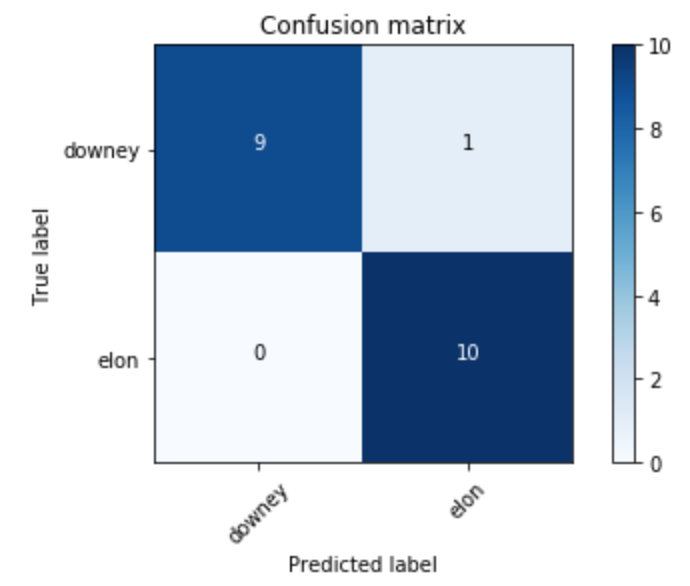
Training over 10 epochs we get to an accuracy of 95%. The confusion matrix below shows that our model is now getting all photos of Robert Downey Jr correct in the test set and is only tripping up on a single photo of Elon Musk.
Figure 4: Confusion Matrix shows accuracy of Binary Image Classifier
The complete notebook for the Single Label Image Classifier is available here
Week 2: Multi-Label Classification - Breaking into the Top 20% of the Kaggle Seedlings Competition
While the previous Resnet34 model was used for single label classification, an image is either an image of Elon Musk or it isn’t, a larger architecture ResNet50 (also described in the paper by Kaimeng He) is shown to have greater accuracy when used for multi-label classification. Here I entered the Kaggle plant seedlings competition to distinguish between twelve different species of plant seedlings based on their images. I trained a ResNet50 classifier on a training set of labeled images and used that classifier to identify plants on unlabelled data.
The biggest difference between the images in this competition and in the previous example are that they would not have been part of the ImageNet database. When looking at photos of plant seedlings, satellite photos of earth or X-rays there are a few enhancements we can make to the image to improve our classification accuracy performance:
- Larger Architecture
- Top-down augmentations instead of side-on
- Masking the image
Instead of relying on the pre-trained ResNet34 architecture that was optimized for ImageNet like data (include facial recognition) larger architectures such as ResNet50, ResNext50 and ResNet101 may prove more accurate.
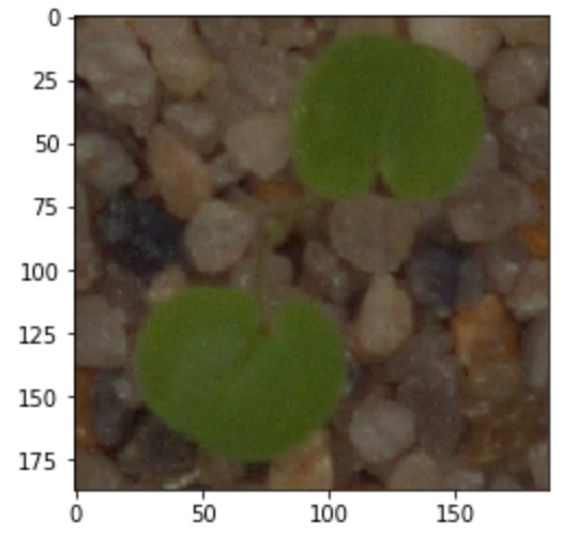
This time our final activation layer is not a sigmoid function as we’re trying to distinguish between 12 plant seedling categories. Instead we use a softmax layer as the final activation function. As a result the final output is as 12x1 vector for each image where the value of the vector is highest for a particular class of a plant seedling.
Figure 5: Top Down Augmentation of Plant Seedlings
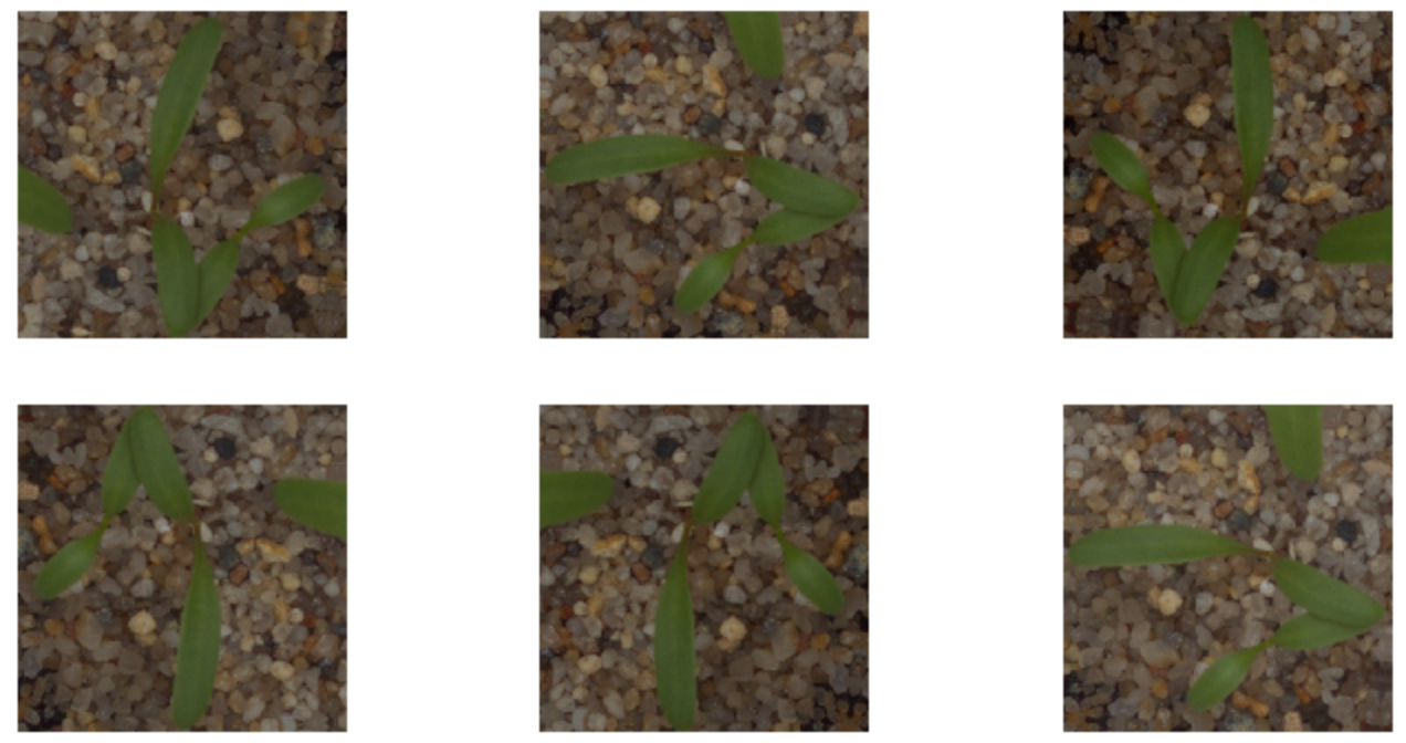
Once again we perform augmentations on the phots of the plant seedlings to give our multi-label classifier more data to work with. However, as our dataset is comprised of photos taken from the top, similar to satellite imagery, we now use top down augmentations on our original images. We are able to reach ~98% classification accuracy on our test set and even place in the top 20% of an Kaggle competition.

Figure 6: Masking the Image Data

A final transformation I explored, which ultimately didn’t add to the classification accuracy was masking out the non-plant portions of images. At a crude level this is equivalent to removing anything not ‘green’ from the image and focusing on the shapes of the green images. I used the opencv library to mask away any “noise” from the shapes of each seedling.
The complete notebook for the Multi-Label Image Classifier is available here and the notebook where masking is implemented can be found here
Week 3: Deep Learning for Structured Data
The first two weeks of the deep learning course focused on unstructured data such as images. In Week 3 we began examining the applications of Deep Learning to structured (tabular) data. The biggest takeaway was the use of embedding matrices to account for various categories of structured data. I used the fast.ai library to tackle the Kings County Housing Data data, relying on the root mean square error as the performance metric. I contrasted the performance of Deep Learning here against more traditional machine learning models and found the best performance came from the use of Extreme Gradient Boosting trees on the test set.
| Model | RMSE on Test Set |
|---|---|
| Embedded Deep Learner | 0.3030 |
| Lasso Regression | 0.2158 |
| ElasticNet | 0.5088 |
| Light Gradient Boosting Model | 0.0126 |
| Extreme Gradient Boosting Model | 0.0081 |
The complete notebook for the structured data on the Kings County Housing Data is available here