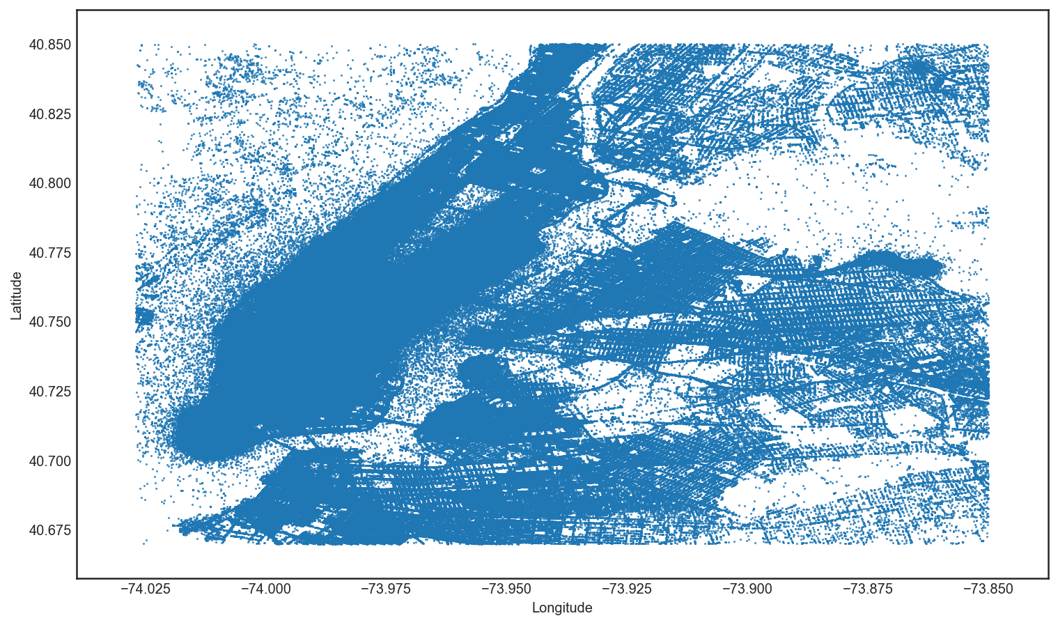
Scatterplot of all pickups and dropoffs in New York City

Summary

This post explores a subset of the NYC taxi dataset for the month of April 2013. I extract, transform and load the trip fare and trip details csv files into a sqlite database. I use this data to predict the fare and tip taxi drivers will receive. The repository containing my entire analysis is here and the presentation slides are available here as pptx and here as pdf.

ETL

The April 2013 taxi data is provided in two csv files: trip_details and trip_fares. I extract, transform and load these csv files into two separate tables: trips_table and fares_table in a SQLite database. I make subsequent calls to these tables in my EDA and modeling notebooks. The ETL process is detailed here.

Data Cleaning

Each table is cleaned for outliers including restricting latitude and longitude co-ordinates to lie in beween (40.67, -74.027) and (40.85, -73.85). I remove trips that last for 0 minutes and 0 miles. I also restrict the dataset to all trips made within New York City alone and it’s two closest airports: La Guardia and JFK International. This excludes trips made to Westchester and Nassau counties (Rate Code 4) as well as out of town trips (Rate Code 5) which are negotiated at a flat fee, where the odometer or trip time is not indicative of the distance or duration of the trip. While these actions may bias the results, 99.84% of all trips in April 2013 were made within the city of New York. A few thousand trips have their payment registered as ‘Disputed’, ‘No Charge’ or ‘Unknown’. These trips were excluded as overwhelmingly, passengers paid by credit card or cash. Finally, the NYC Taxi and Limousine company permits a maximum of 6 passengers in a 5 passenger taxicab, if the sixth passenger is a child under 7 who can sit on an adult’s lap. I screen out all trips with more than 6 passengers.

Data Merging

Using taxi medallion as unqiue taxicab identifier, hack license as unique driver identifer, vendor id and pickup_datetime as common keys, I merge the two tables above and return just over 14 million rows of data. Going forward, I use the assignment questions to propel my EDA of the dataset. The complete data munging process is described in this notebook.

Basic Questions

Complete notebook available here.

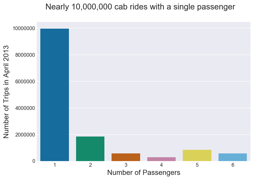
Q1. What is the distribution of the number of passengers in each cab?

Overwhelmingly taxi cabs are hailed by a sole passenger. More cabs are hailed by a single passenger than the total number of cabs hailed by two or more passengers as shown in Figure 1.

Figure 1

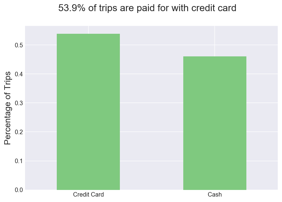
Q2. Do most customers pay with cash or card?

The results are pretty close, with nearly 54% of trips being paid for by credit card.

Figure 2

Q3.1 What does the distribution of fare amounts look like?

The initial charge on a cab is $2.50, so I confirm there are no fares below this amount. The most expensive fare was $204 while most fares were under $35.

Figure 3

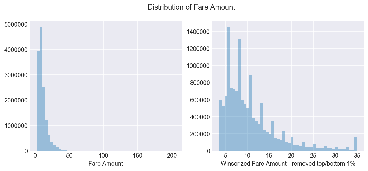
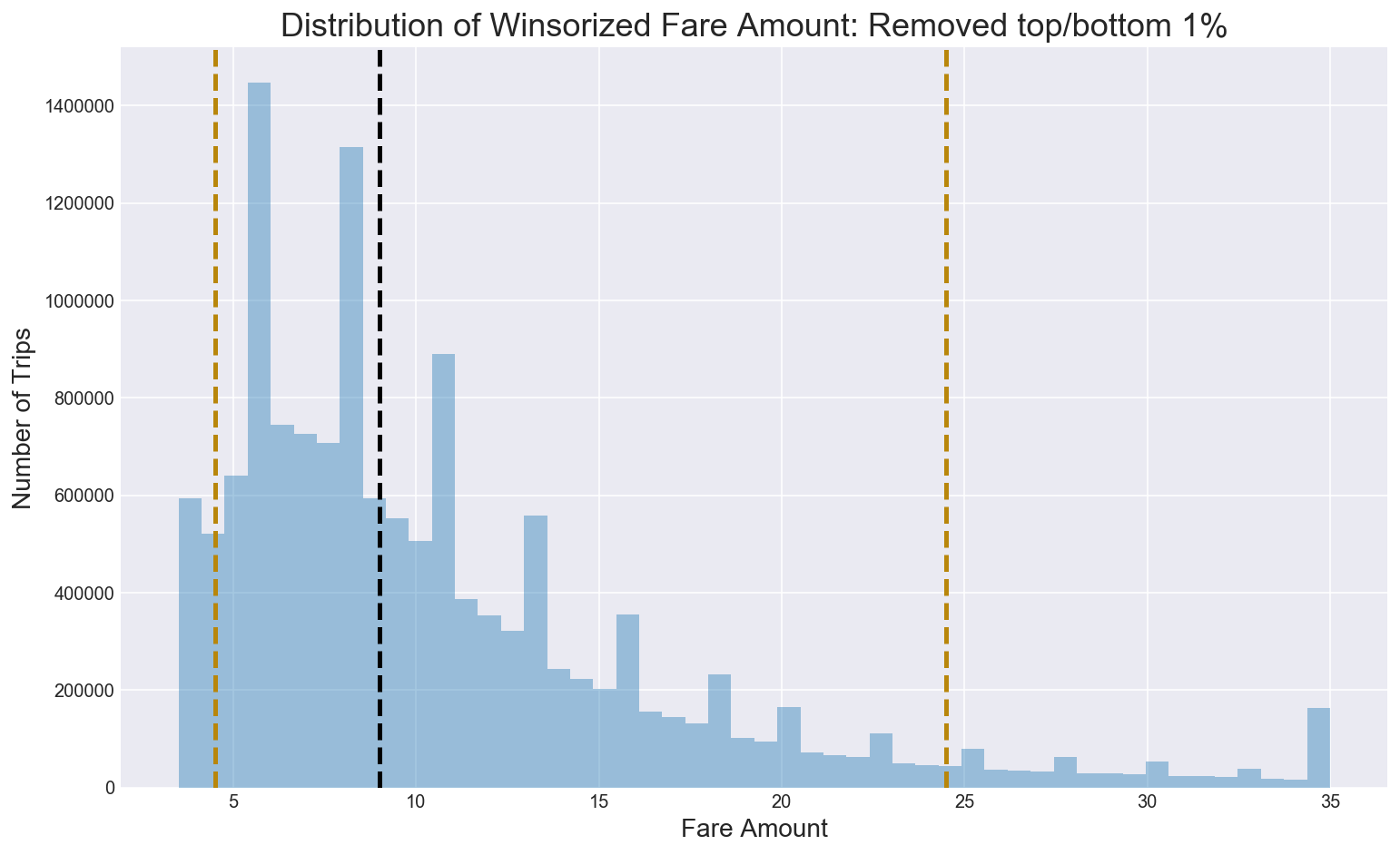
Winsorizing the fare amount data by removing the top and bottom 1% shows the median fare amount is $9 as shown below. The bottom 5% of fare amounts is less than $5 while the top 95% of fares is higher than $24.

Figure 4

3.2 Is there a difference between airport and non-airport fare amounts?

Figure 5 shows the median and modal airport fare amount is $52. This is in contrast to non-aiport fares which tend to be under $35.

Figure 5

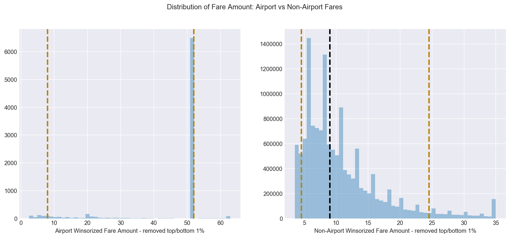
I looked into whether this specific fare amount was more or less likely to be paid by cash or credit card but the results were split with 56% of passengers choosing to pay with card and 44% choosing to pay with cash.

Q4.1 What does the distribution of tip amount look like?

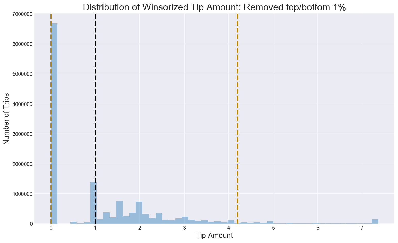
When looking across all rides, most passengers don’t appear to tip well. While tip amounts via credit card can be verified, cash tips may be underreported by the taxi drivers themselves. Winsorizing the distribution of tip amounts, the modal tip amount is $0 while the median is $1.

Figure 6

Q4.2 Is there a difference in the distribution of airport versus non-airport tips?

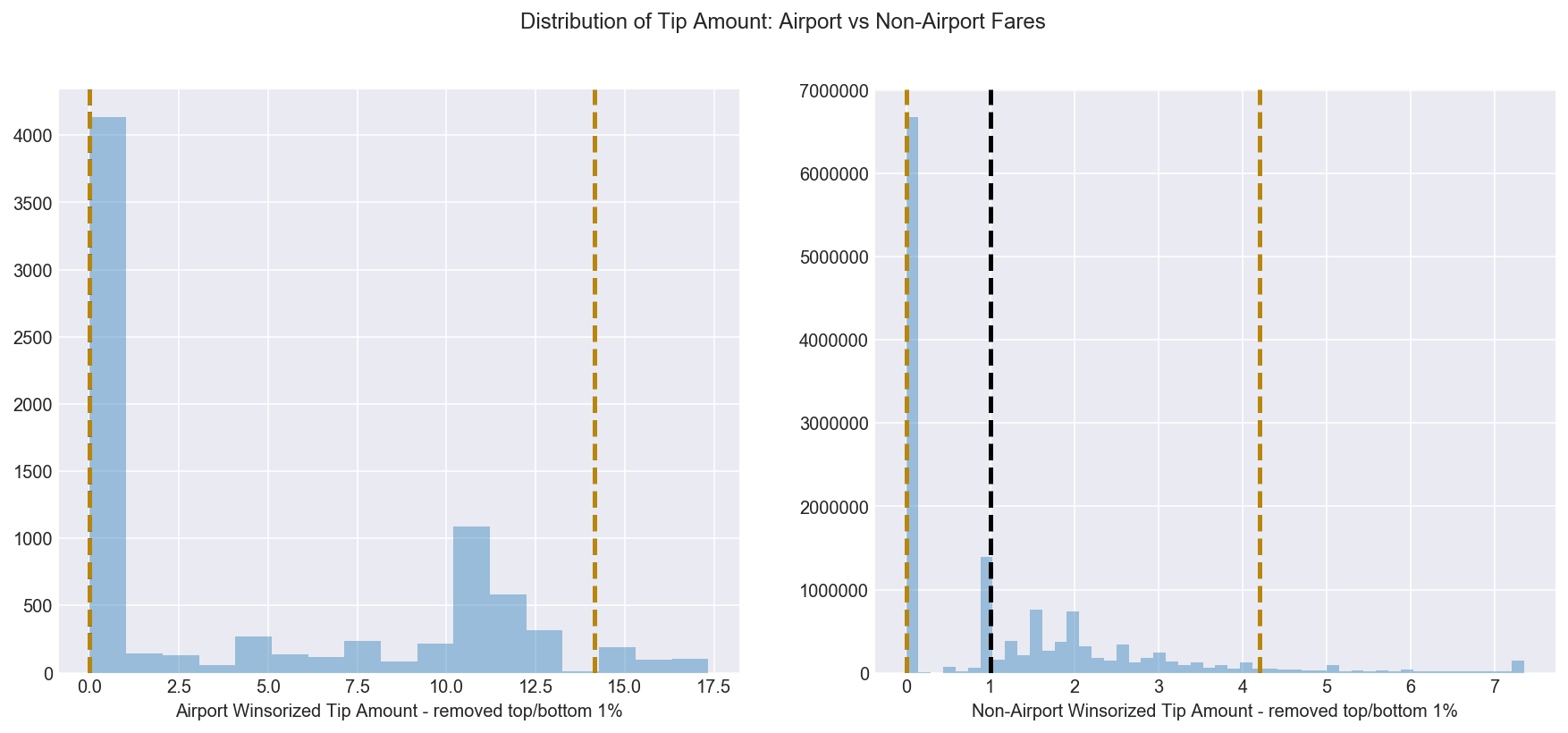
However, passengers tend to be more generous when it comes to tipping the cabbies that take them to the airport. Even though there are fewer airport fares compared to non-airport fares, it is understandable that drivers would want to take more airport trips.

Figure 7

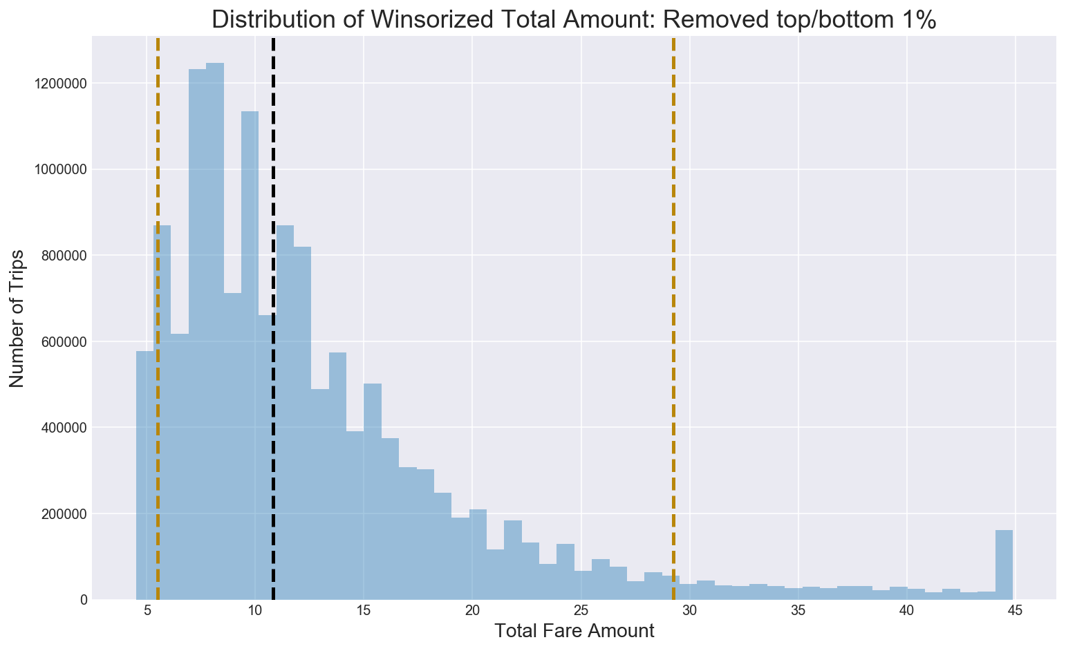
Q5.1 What does the distribution of total amount look like?

Given the relatively low tip amounts reported, the distribution of the total amount will be similar to the distribution of the fare amount. Winsorizing the total amount by removing the top and bottom 1% shows the median amount is just shy of $11.

Figure 8

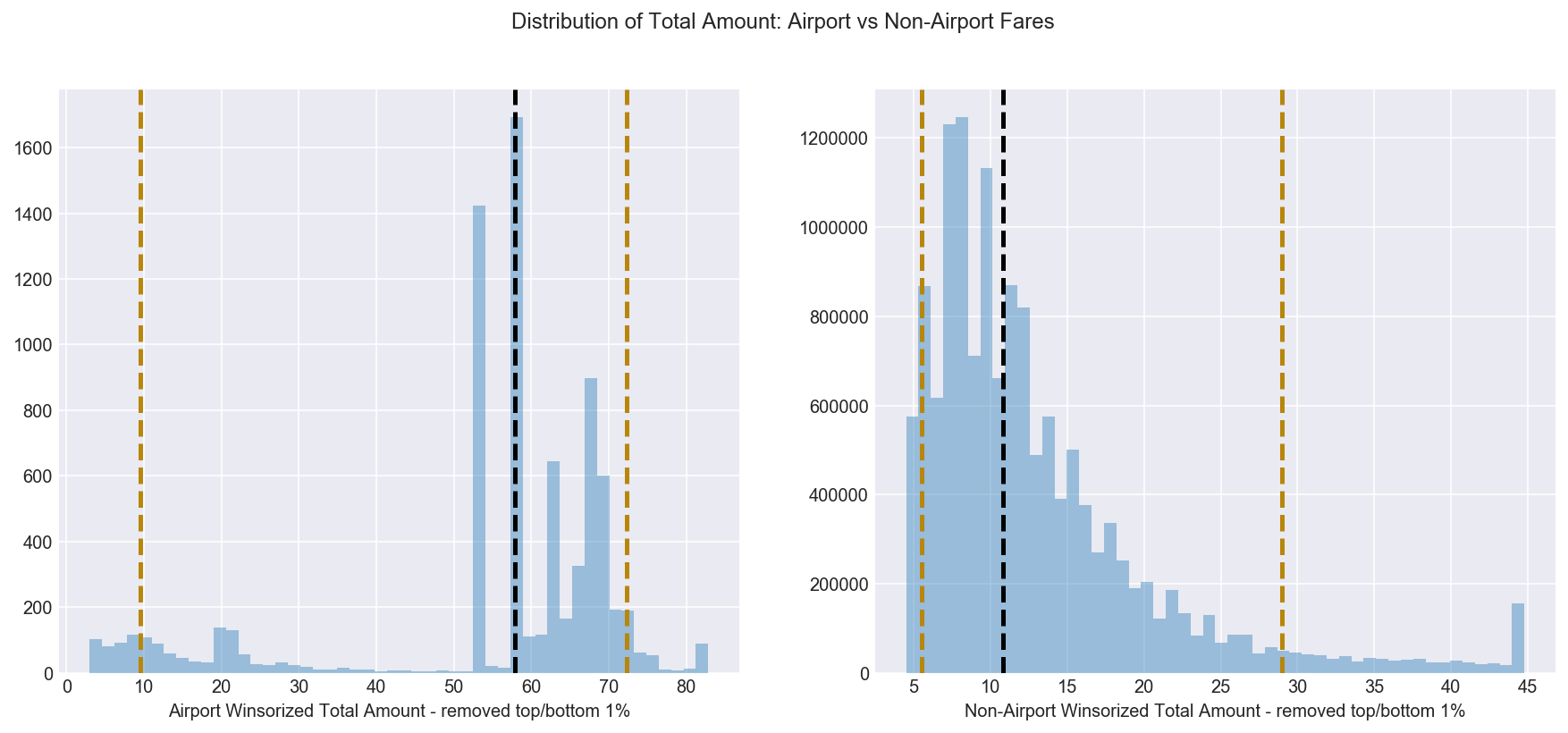
Q5.2 What does the distribution of total amount look like?

Airport total amounts are higher than non-airport total amounts which makes sense as airport fares are higher than non-airport fares. The median/modal airport total amount is $57.83.

Figure 9

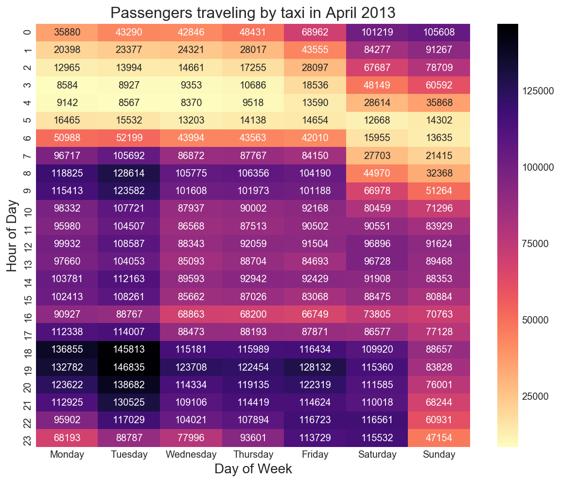
Q6. What are the top 5 busiest hours of the day?

Evenings after work or dinner appear to be the busiest which most cabs being hailed at 7pm. The heatmap below shows that Monday and Tuesday evenings between 6pm - 8pm followed by Friday and Saturday evenings, are when most taxi trips occur.

Figure 10

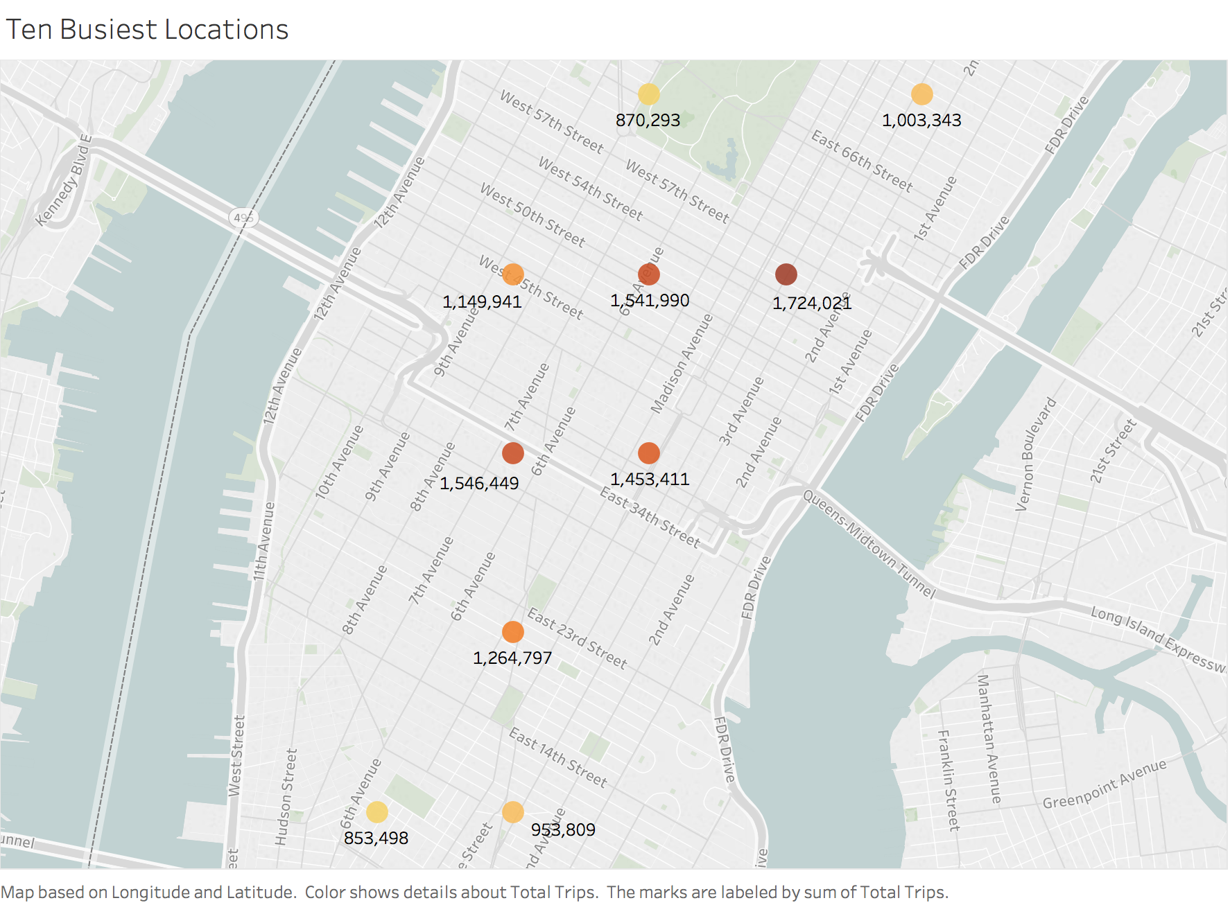
Q7. What are the top 10 busiest locations in the city?

I filter latitude and longitude down to 2 decimal places and then sort through the most popular pickup and dropoff locations. These are identical and are all located in Manhattan, over 12.36 million trips. Rounding down latitude and longitude will increase clustering of pickup and dropoff points.

Figure 11

Q8. Which trip has the highest standard deviation of travel times?

Each trip is uniquely defined by its pickup and dropoff co-ordinates. It is important to determine what minimum sample size of trips to use to calculate the standard deviation. If there is a unique trip for example, then we cannot calculate it’s standard deviation of travel times. What minimum sample size do we need to determine the standard deviation of trip times? If there is a trip that has occured twice, one trip being 5 minutes long and one trip being an hour long, this trip will have a very high standard deviation based on a relatively small sample.

I make the following assumptions:

1. Margin of Error = 5%
2. Confidence Interval = 95% which is a Z-Score of 1.96
3. Standard Deviation = 0.5 (expecting 50% standard deviation will ensure large enough sample size)

The required sample size = ((1.96 x 0.5)/0.05)^2 = 384.16 = 385 trips, which is the minimum threshold of trips applied. All routes with fewer than 385 trips over the month are excluded. This minimum exclusion is applied to answering all questions going forward.

Figure 12

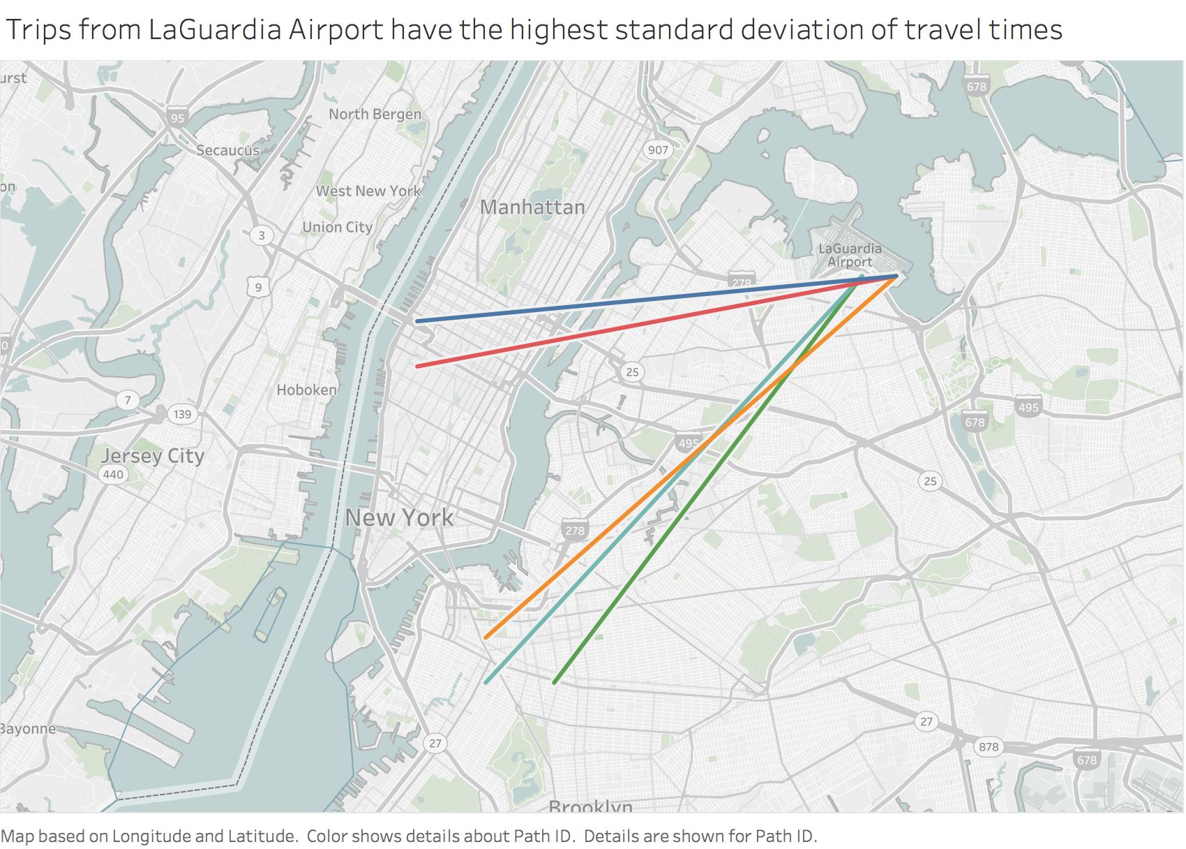
Travel times for trips originating from La Guardia airport to New York’s boroughs have the largest variance. Apparently airport traffic IS a nightmare.

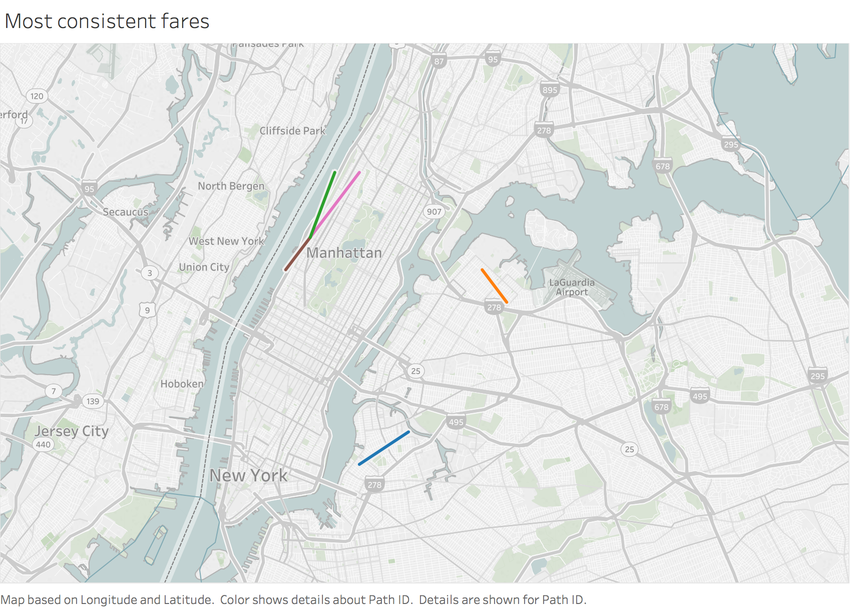
Q9. Which trip has the most consistent fares?

Using the same minimum sample size threshold, I now examine the top 5 fare amounts have the lowest standard deviation as these will be the most consistent fares. Figure 13 reveals that these are shorter non-Airport routes. Three of these trips begin at the same location in Manhattan. To get more color on the differences between trips it would be interesting to understand the time of day and day of the week the trips were occcuring on.

Figure 13

Open Questions

Q10. Which trips can we confidently use means as measures of central tendency to estimate fares, time taken?

As mentioned in question 8 above, certain trips may only occur once or twice, making calculations of central tendency based on these trips biased and erroneous. If the same trip takes twice as long for one taxi driver as it does for another, and our population is two trips, this skews calculated means and variances.

So how many occurences of the same trip - identified as beginning and ending at the same geocodes - are required before measures of central tendency can be calculated with confidence? Among 14 million trips, should the threshold be 50 occurences of the same trip or 1000?

I make the following assumptions:

1. Margin of Error = 5%
2. Confidence Interval = 95% which is a Z-Score of 1.96
3. Standard Deviation = 0.5 (expecting 50% standard deviation will ensure large enough sample size)

The required sample size = ((1.96 x 0.5)/0.05)^2 = 384.16 = 385 trips, which is the minimum threshold of trip occurence over the month to be comfortable calculating measures of central tendency to estimate fares. Most of the trips which originate and end in Manhattan, including trips to La Guardia or JFK airports cross this threshold easily.

Q11. Build a model of Taxi Fare and tip given pickup and dropoff location

Fare modeling notebook available here while the tip prediction notebook can be found here.

I examine the correlations between trip fare (and log fare) versus the features in my database. It stands to reason that several features will have a high correlation with the fare including how long the trip was and the distance covered.

Figure 14

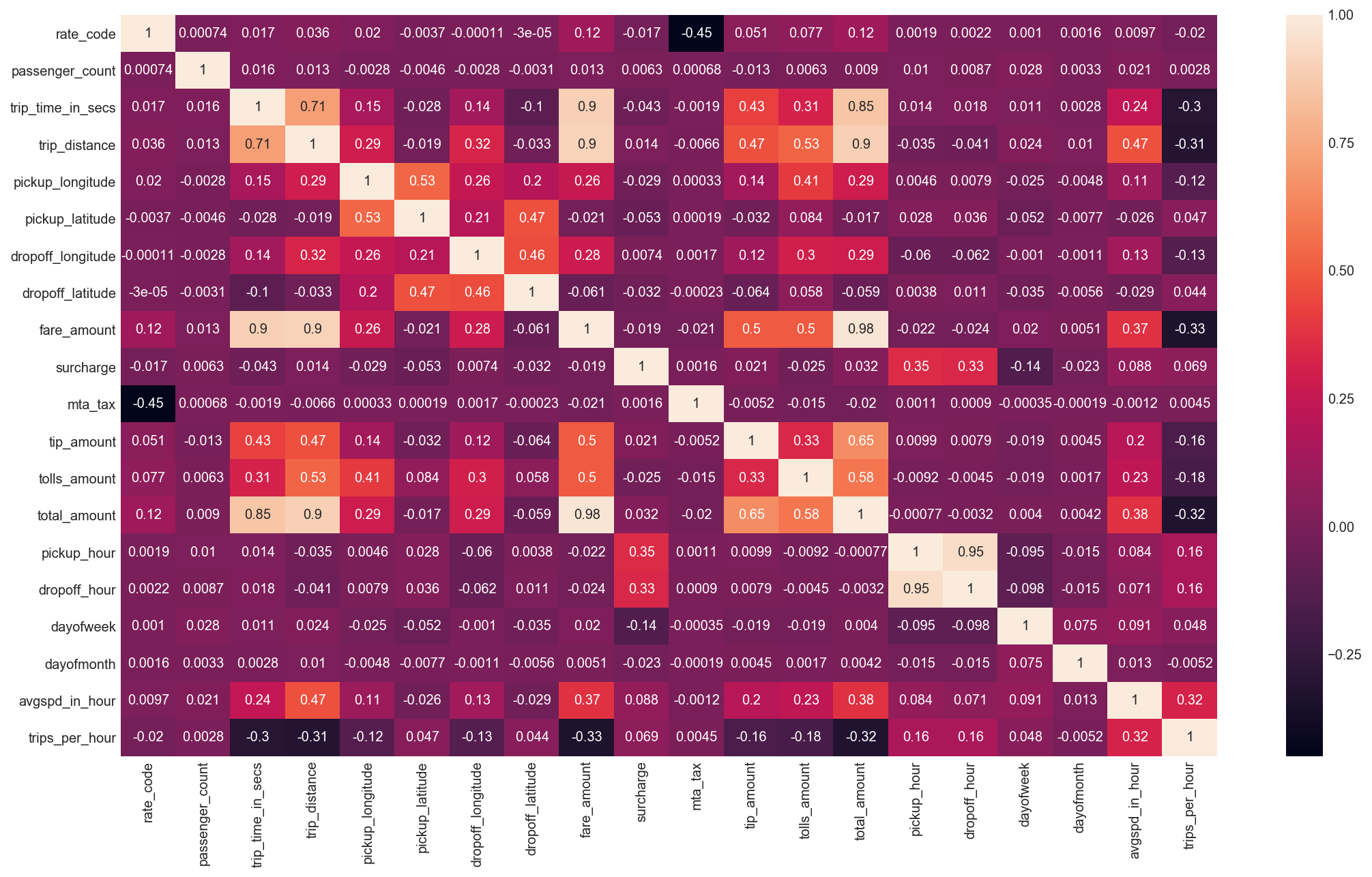
The variables chosen to predict fare and percentage tip include:

1. Average Speed Each Hour
2. Trips per Hour
3. Pickup Longitude and Latitude
4. Dropoff Longitude and Latitude
5. Trip Distance
6. Pickup Hour
7. Dropoff Hour
8. Day of Week
9. Day of Month

As there are millions of data points I use as RANSAC Regression model using the 9 features above as it is robust to outliers in the y-axis. The model has an R-square of 80.7%. The OLS model has a slightly higher R-square of 82% which persists after running a five fold cross validation. I show a line of best fit among the fare data in Figure 15 below.

Figure 15

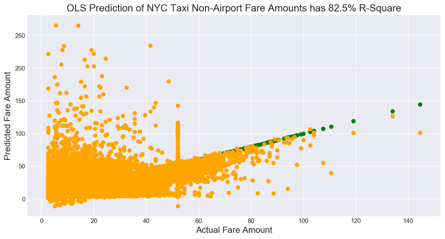
Note the scatter plot of predicted versus actual fares shows a cluster of fares at the $50 mark, which requires further investigation. Either these fares were rounded or mis-reported by the taxi drivers. It may seem obvious that taxi drivers may negotiate lower fares up to $50. What is more puzzling are fares where our linear model predicts a high fare, but the taxi driver only reports $50. Are drivers pocketing these large fares?

Figure 16

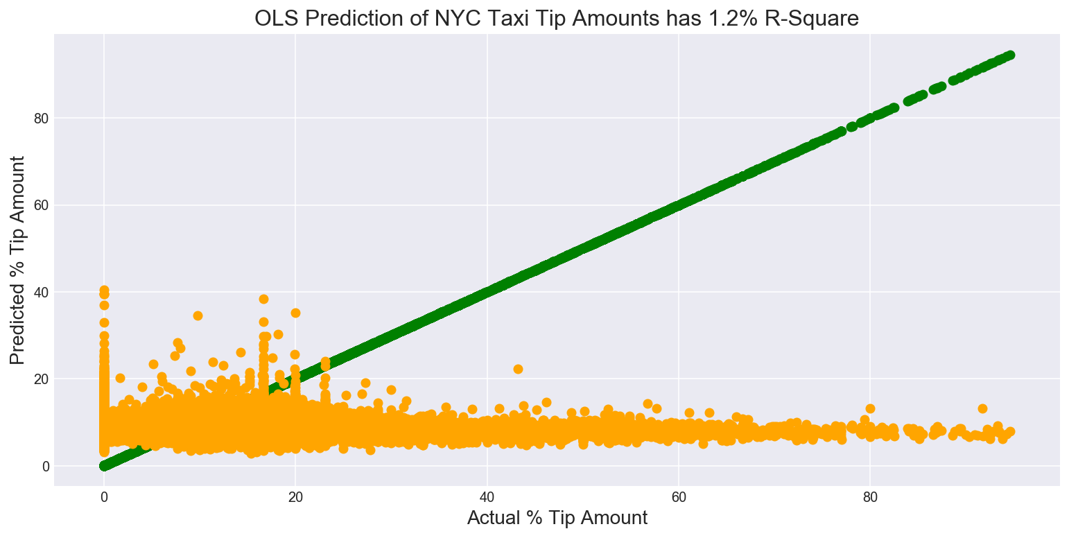
When it comes to predicting the percentage of the fare that will be left as a tip, I use a similar linear model. This time an OLS regression has an R-square of 1.2% when it comes to predicting how much of the fare will be a tip. The linear model does a very poor job of predicting the percentage tip amount. We fare slightly better using a Neural Network and a Random Forest Regressor.

Q12. How would a taxi owner maximize earnings in a day?

I distinguish between a taxi owner and a taxi driver as follows. The taxi driver is represented by the hack license and their average daily earnings in April 2013 was $259 a day. A taxi owner owns the medallion for a given taxi and can have several drivers drive their cab. The average daily earning by a medallion (taxicab) was $480 per day.

The average daily revenue for taxi drivers is $480 per day. The constraining factor here is driving hours per day. I consider two approaches: looking at routes that generate the highest daily revenue and the routes that earn the highest revenue per hour. This way a taxi owner can either concentrate on areas that generate the highest revenue or lease out a medallion taxi to two drivers driving 12 hour shifts to maximize daily revenue.

Figure 17 plots all routes that generate that highest daily revenue and the total number of trips required to generate this revenue. Note all these trips are all based in Manhattan, except for one which is from Manhattan to La Guardia Airport.

Figure 17

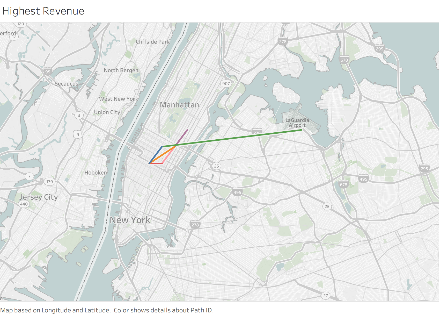
Note from question 8, the trip to LaGuardia airport has the highest standard deviation of travel times. As total amount charged will vary will the time of the trip, consistently relying on this trip for maximizing revenue may not be the best solution. A taxi owner could prioritize taxi bookings for Manhattan trips and potentially take on other trips if they crossed the average daily revenue of taxi drivers ($480).

Another way to consider this problem is that we are trying to maximize revenue in the available time. I build a feature which is the ratio of total_amount/time driven in hours and see which routes maximize the earnings per hour driven. These routes can be maximized upon. Note assumptions here are that regardless of time of day these are the most profitable routes per hour.

Figure 18

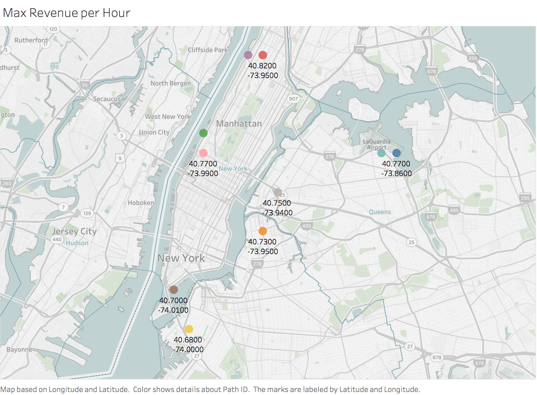
Interestingly, these trips begin and end at the same geocode (rounded to 2 d.p.) and there appear to be intra-Manhattan geocode or intra-Airport geocode trips. These shorter trips can be used to maximize daily earnings. The results when trying to maximize the total amount earned per mile driven are identical.

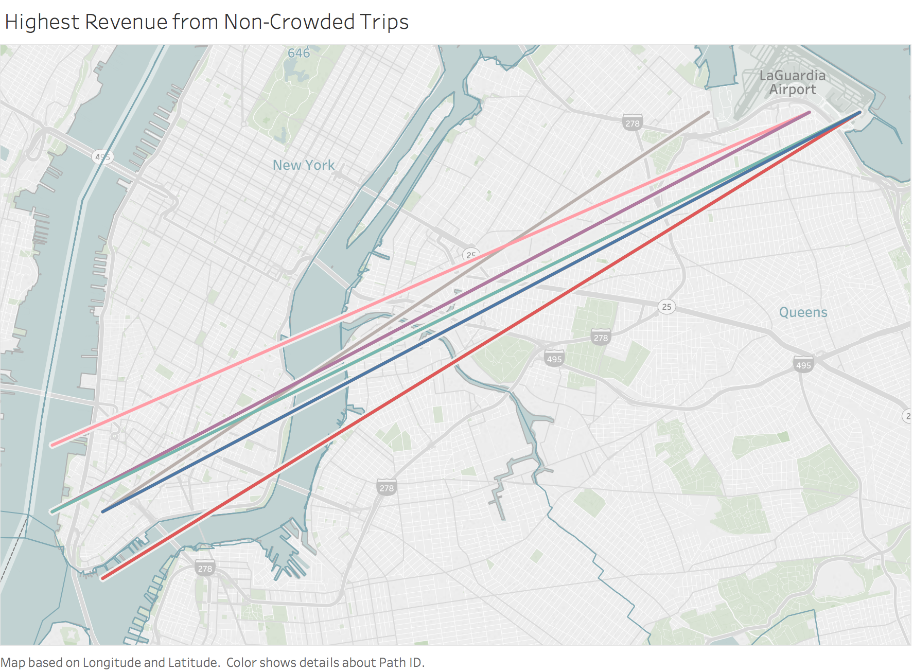
It may be unrealistic to expect taxi drivers to keep driving back and forth between the same set of streets all day. In this case it may bear looking at less crowded routes as discussed in Q14 below.

Q13. How would a taxi owner minimize work time while retaining average wages earned by a typical taxi in the dataset?

As mentioned above, the average daily earning of a taxicab is $480. Looking at Figure 11 again, note that demand for taxicabs highest on Monday and Tuesday evenings between 6pm - 8pm or Monday and Tuesday mornings between 8 and 10 am. This is the morning and evening office traffic.

Figure 10

A taxi owner looking to minimize their driver’s work time should ensure drivers are working the morning rush and evening shifts from 6pm onwards. By contrast demand for taxis is much lower between 3am - 5am Monday to Thursday, so these hours can be skipped over.

By far the evening route that generates the most revenue per hour begins and ends from geocode (40.77, -73.86) and is an airport to airport transfer route. These are followed by several routes within Manhattan and are shown in Figure 16 below.

Figure 20

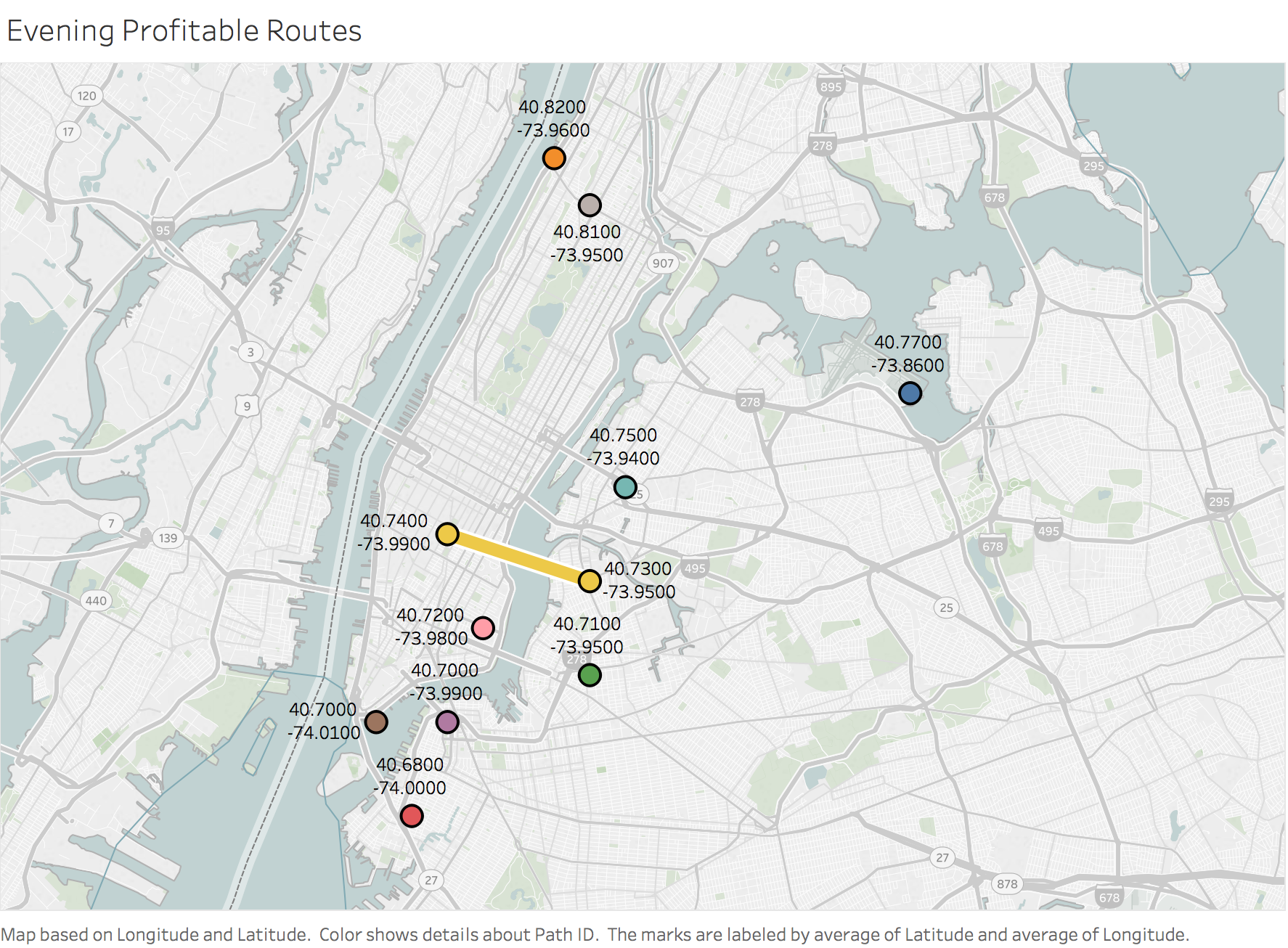
These evening routes generate the highest total fare amount per hour of driving. Taxis can focus on these locations until they hit their daily goal of $480 (or $259 per driver). After clearing their goal they can move on to more varied fares. Alternatively, if a taxi driver started off at a location other than the ones highlighted in Figure 16, they can drive to these routes to make up their daily fares.

Q14. How would a taxi company with 10 taxis, maximize earnings?

Assume each taxi can be driven all day by 2 drivers working 12 hour shifts without wear and tear. This translates to 20 shifts per day for the taxi company. I would ensure taxis are available at the most popular pickup and dropoff locations and for trips with the most consistent fares. However you wouldn’t want taxis working for the same company to undercut each other for the same fare.

My analysis so far reveals several insights for a smaller taxi company:

a. Instruct taxi drivers to focus on the routes with the highest earnings per hour (or earnings per mile). This would keep taxis working within smaller areas (zipcodes) and would allow the company to keep a fleet of cars working airport shifts and another fleet working Manhattan island shifts. The difficulty here is whether taxis could legally deny providing service to passengers who want to travel out of these zones

b. Once a taxi driver has earned half the average daily wage of taxi driver ($240) during their shift, give them the option to engage out of town fares or those fares whose trip times have higher standard deviation e.g. Manhattan to LaGuardia fares or possibly out of town fares where the total amount earned may be higher.

c. The worst time to have a taxi out for service are weeknights or Friday and Saturday nights as these tend to be the busiest times. Get taxis serviced during the day.

d. The most popular routes may be overcrowded, so it may be worth focusing on trips that generate the highest total revenue with the smallest number of individual trips, as shown below.

Figure 21

Further Questions

It would be interesting to see the impact of services such as Uber or Lyft on taxi demand over time. Also of interest would be the impact of precipation or temperature on a particular day on taxi demand, fare and tip. Finally, information on traffic congestion and road conditions would be invaluable to getting more insight from this dataset.